Literature course

This post covers chapters 18, 19 & 20 from Futuyma and Kirkpatrick’s book on Evolution (2018). The author of this post is Jacqueline Hoppenreijs.

We’ve heard all about the appearing and disappearing of species and species groups on and off the Earth’s surface over the past billions of years…So now it’s time to see how these are linked to the changes that the very surface itself has seen and zoom out a bit, both in space and time! 

The geography of evolution

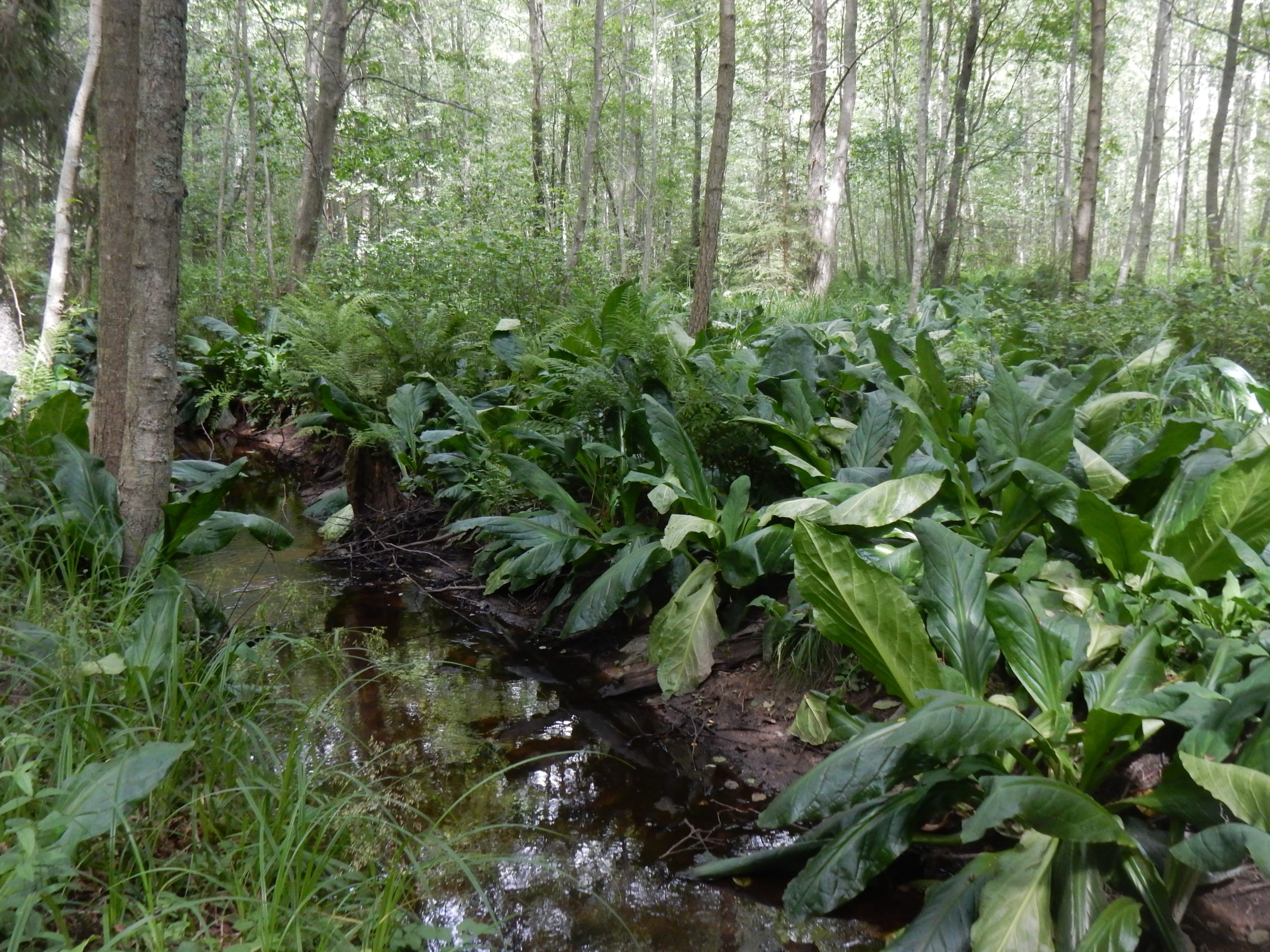
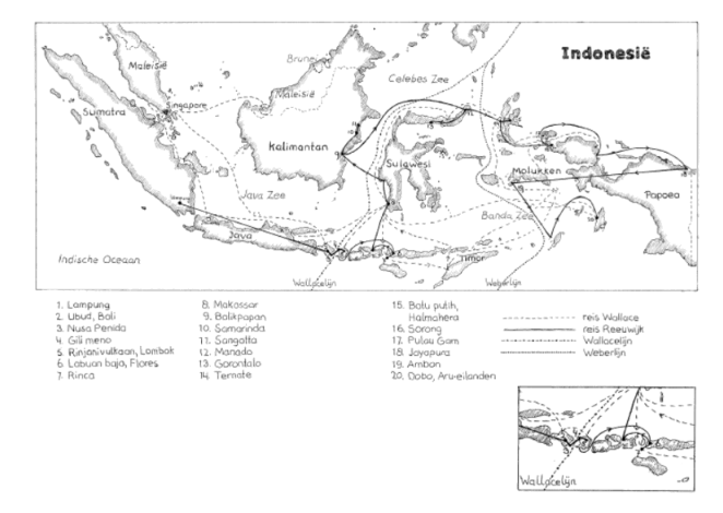
Linking the geographical distribution of species to their ecology is called biogeography, a field that started with the extensive travels of Alexander von Humboldt. He was one of the first to try and figure out why a species occurs in one place but not in another, leading to research on the traits that enable species to live in specific places, measurements of environmental characteristics and, eventually, species’ evolutionary history. Charles Darwin, who was an enormous fan of Von Humboldt (Wulf, 2015), was the first to describe how physical barriers lead to different species occurring in different places, and how similar traits develop if those places are similar. While he was exploring South America, his colleague Alfred Russel Wallace made similar discoveries in south-eastern Asia and Oceania. Following that, Wallace developed a model of biogeographic realms: regions that are inhabited by similar plant and animal taxa. Knowing about the Earth’s geological history, one realises that the current geographical distance between localities is far from the best predictor for ecological similarity of species communities. The realms Wallace himself studied most intensively were the Oriental and the Australian lines, separated by what’s now best known as the Wallace line (Figure 1). The islands of Bali and Lombok, separated by this line, are no more than 50 km apart these days, yet the species groups that inhabit the respective islands are different. The Indomalayan biogeographic realm on the west is maybe best known for its large mammals, such as the Javan rhinoceros and Indian elephant, and its diversity in pitcher plants. On the other side of the divide, the Australian realm is known for marsupials, birds of paradise and eucalypts. There are, however, multiple interpretations of potential lines, of which the Weber line probably is the best-known alternative (Simpson, 1977).

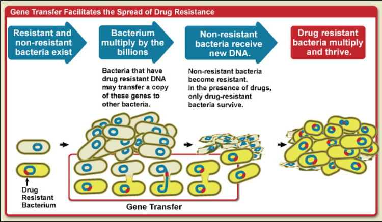
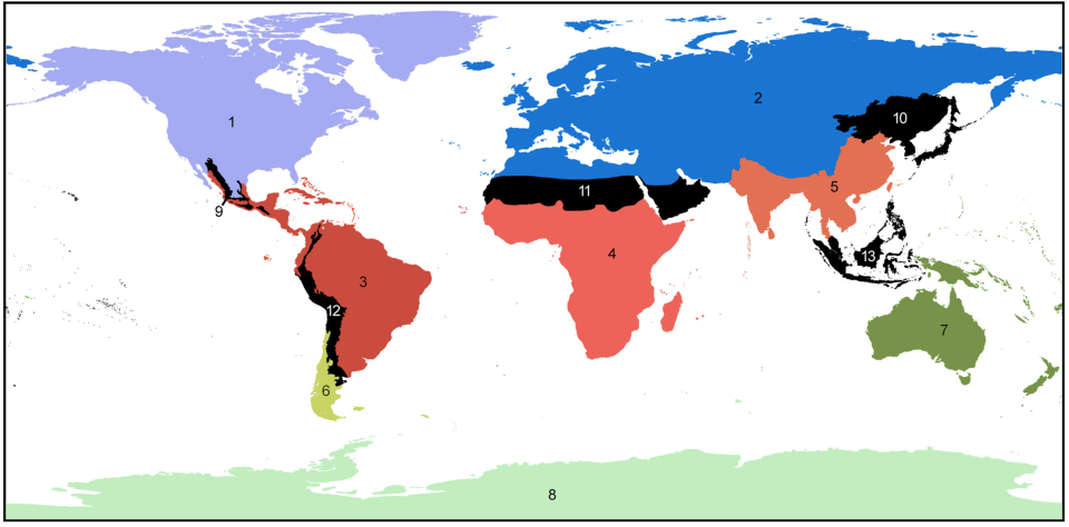
We’ve previously learned about how geographical barriers shape species distributions. While Humboldt, Darwin and Wallace were forced to work with species descriptions and phenotypical measurements, scientists these days have a much wider array of methods at their disposal to map the historical processes of past and current species distributions. The main processes driving these distributions are dispersal, which we have seen can be gradual and look like a stepwise species distribution, and vicariance. Dispersal patterns can, however, also look like giant leaps, for example when a few individuals cover a large distance and start a new population far away from their homes, or when dispersal happened gradually but populations between the two ends of the distribution have been wiped out and gone extinct. This geophysical separation is a form of vicariance, the process that leads to disjunct populations, and often comes in the form of climatological or tectonic disruption. With an increased understanding of plate tectonics and technologies to research fossil remains and build phylogenetic trees, scientists are now able to map the processes driving species distributions better than ever. Our better understanding has led to there being multiple and more nuanced angles to the debate around biorealm delineation, and the general acceptance of there being at least some type of transition zone (Figure 2; Morrone, 2023). 

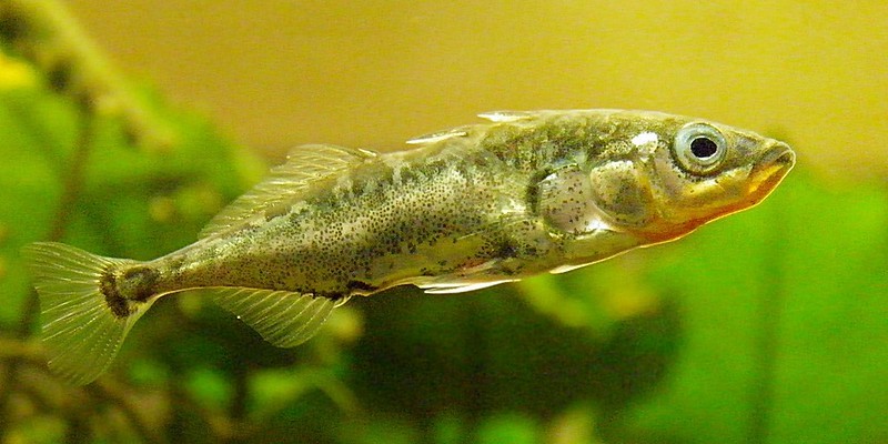
The current distributions of species are a result of these historical processes and current circumstances. The limits of their ranges are decided by several factors, of which dispersal is again an important one: how well is the species able to spread to new areas? That doesn’t only concern the activity itself, but also whether the species finds a mate in this new area (if it depends on sexual reproduction) and how well the species is able to settle in. That means that it needs to be able to find its ecological niche, or in the case of eco-engineers at least to the extent that they can modify it further to fit their requirements. The fundamental ecological niche is the set of abiotic and biotic conditions in which a species finds its most basic needs met, although it might not be the most favourable place. That means that a species A that has its optimum temperature at 17°C but tolerates temperatures between 14 and 24°C, has a niche width of 10°C. Take a species B that thrives at 21°, however, and this species B might outcompete A out of the “upper” part of its fundamental niche. A’s realised niche is thus narrower because of species B, which illustrates the competitive exclusion principle. While this sounds like a relatively modest consequence for species A, it doesn’t sound like a fringe issue at all when you think of the enormous shifts in temperature that the climate crisis causes. Lajeunesse and Fourcade (2023) analysed one of the world’s largest databases, GBIF, on nine different animal taxa and found that almost all of them now consist of species with higher preferred temperatures than 30 years earlier. Since species that are phylogenetically closely related often have similar niches (also called phylogenetic niche conservatism), this means that replacements can be with quite dissimilar species which in its turn can lead to drastic ecological turnovers. Add to the fact that temperature increases are not the only consequence of the climate crisis and the fact that Lajeunesse and Fourcade found that there’s a time lag of these effects too, and we’re looking at a serious problem.

The evolution of biological diversity

While it’s becoming painfully clear that we’re entering the sixth mass extinction (Cowie et al., 2022), it’s not quite as clear how large of an extinction that will be: we simply don’t know how many species inhabit Earth at this time! Current estimations lie between 2 and 8 million eukaryotic species, and we know that those are wildly unevenly distributed in space but also over taxa. It’s not quite clear what drives these differences, but if we’re taking a straightforward approach, we can start by counting species in each of these taxa. If we add information about speciation and extinction rates, we can reason towards a diversification rate, which tells us something about a taxon’s increase or decrease in species richness over time. Two different components of this equation (the time that the taxon has had to undergo diversification and the diversification rate itself), together with the carrying capacity of the system, can help us understand why some species groups are more species-rich than others. A similar argument goes for different areas since areas closer to the equator are usually more species-rich than areas on higher latitudes.

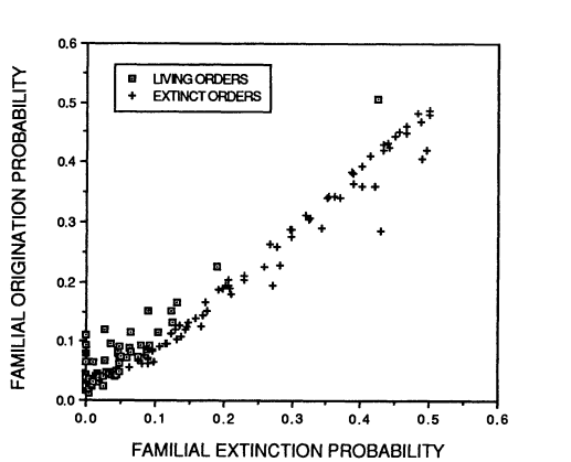
Archaeological records can be used to map past speciation and extinction patterns, and have led to the discovery of, among other things, the Cambrian explosion (which, while sounding violent and destructive, refers to a period of speciation instead of extinction) and previous mass extinctions. The aforementioned sixth mass extinction and its predecessors are not the only time that species or entire taxa became extinct: there is a usual background extinction rate that makes all geological strata potential sources of now-extinct specimens. Both this background extinction rate and the speciation rate have generally declined over the past hundreds of millions of years, and it’s not quite clear why. Especially extinctions should be random, and thus extinction rates quite constant since they depend on random environmental variation and natural selection. Alternative hypotheses are 1) species-rich taxa don’t count as extinct until all of the species within the respective taxa are indeed extinct, and right now we happen to have a lot of species-rich taxa, and 2) the taxa that undergo rapid speciation and extinction are mostly extinct now, and we’re left with the taxa that go through these processes more slowly. The second hypothesis builds on the fact that speciation and extinction rates of taxa are correlated with each other (Figure 3).

While scientists have found out that extinction rates are relatively constant per taxon, mass extinctions were everything but random: some taxa had better chances to survive than others. Their respective chances depended not on the usual factors, such as consisting of many species, being widely distributed and so on, but on specific characteristic X that allowed them to deal with the cause of mass extinction Y (or not, obviously). One could thus say that evolutionary change works on three levels here: there’s the level of change within species or even populations, the level above on which species originate and go extinct at normal rates a.k.a. species selection, and the final level in which mass extinctions reshape the whole landscape of flora and fauna.

Reshaping consists not only of the wiping out of large parts of species communities, but also offers the opportunity for species to take in the niches that newly opened up and that are relatively competition-free. Mass extinctions are often followed by higher speciation rates, especially if a key adaptation comes to life. Key adaptations are species characteristics that open up a whole new niche, think of the wings of insects that opened up the possibility of flight or lignin in plants that allowed them to build more sturdy structures and colonise land. Such adaptations can lead to increased speciation rates or even periods of radiation, which can result in bouncing back to a certain equilibrium of species richness. Whether such equilibria exist is, however, a topic of discussion, and certainly also depends on the spatial scales one looks at. Local richness can depend on regional richness and is to a certain extent limited by resource availability and competition levels, since higher species diversity tends to lead to lower diversification rates. If not a perfect equilibrium, these dependencies at least suggest a certain bandwidth wherein species numbers fluctuate. If we zoom out, however, we also see how new taxa take in open ecological spaces, suggesting ever-increasing diversity. With that, we can safely assume that there are at least some among us that will have an answer to the sixth mass extinction.

Macroevolution: evolution above the species level

As we have seen for extinctions and speciation, processes don’t always have to be gradual and through small steps. The same seems to be true for evolution: while many changes are small and gradual, there also seem to be sudden developments of characteristics. The field of macroevolution covers these and related questions, such as whether such leaps are as random as small mutations. Evolution above the species level, also called macroevolution, shows surprising parallels with evolution within species (microevolution).

Such parallels include intermediate steps on the level of whole taxa instead of single species; intermediate steps that lead to completely new life forms. Examples are the dinosaur fossils that had feathers long before their carriers were able to fly; these feathers were mainly for insulation. It was only when other characteristics, such as smaller body sizes, changed that we would see animals that started to resemble our modern birds. The same goes for mammals: the skulls that allowed for strong jaws and large brains developed step by step and can, due to the nature of the material, be traced back with the help of fossils.

Such fossils can help us fill the evolutionary gaps between related taxa, for example between whales and other mammals. Now-extinct intermediate species could display different degrees of being amphibious, reduced teeth or moved nostrils, and explain roughly how and when four-legged land mammals went “back” to the sea. Some steps that we know about now seem so large, that some rather call them leaps or saltations. Some researchers have even gone as far as calling the few surviving products of these supposed saltations “hopeful monsters”.  Often, however, these monstruous leaps are merely lacking proof of intermediate steps in our fossil record.

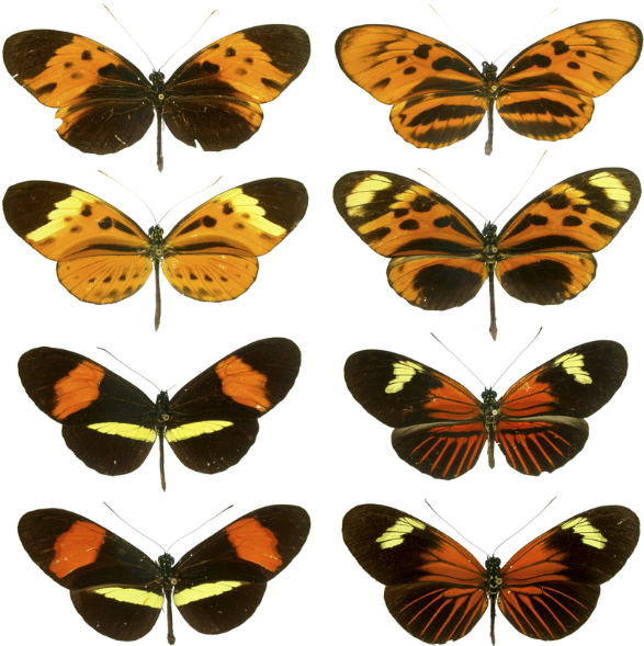
All of these steps have something in common. They’ve either been an adaptation to the environment that its carrier could benefit from, or they’ve been a by-product of the adaptation or a random change that didn’t have negative consequences to the extent that they were selected against. The latter may also become beneficial characteristics, with changed circumstances. Adaptations sometimes follow behaviours, such as when species change their feeding behaviour, and can be shaped by modifications without a direct genetic basis during an organism’s development. The complexity of phenotypes that we see today is, to some, enough ground to say that a special someone or something has had a hand in creating all these so perfectly working organisms. Unfortunately for them, our understanding of past steps, both small and (seemingly) large, proves that complexity is no reason to assume creation, rather that complexity might be caused by passing time and adaptive evolution through natural selection. For those that need more convincing, the similar changes that we see evolve independently from each other when taxa adapt to similar living conditions should do the job. Such adaptations are similar in function but clearly have different evolutionary origins, and are called analogous. Their conceptual opposites, homologous adaptations are generally speaking adaptations that have different forms across taxa, but are inherited from a shared ancestor. Biological homology is a bit broader than this, as it includes any characteristic that develops through a similar developmental pathway, i.e. eyes or extremities.

As we now know, the rate of evolution can be wildly different over time, between taxa, and so on. It is measured as an amount of change, for example in a mean trait value, per unit of time. What is tricky about this calculation is that its outcome is usually high when measured on a short time interval, and low when measured over a long time. That’s because of the loss or reversal of newly acquired adaptations, but also because of the previously mentioned niche conservatism.

With so much knowledge about the past under our belt, dare we look into the future? It’s safe to say that the processes that have driven evolutionary change in the past will continue to do so, but their direction and the extent of their respective effects is less clear. It’s possible to discern trends though: changes in a certain direction, that, for example, can be measured through the aforementioned mean trait values. Traits that follow passive trends are equally likely to develop in either direction, whereas an active trend means that development in one direction is more likely than in the other. Trends can become passive or active in a certain direction because of individual selection, speciation or extinction rates and species selection. Two major trends that we can distinguish are those towards higher efficiency and higher complexity. The former can be measured in, for example, the amount of energy it takes to perform certain functions. The extent to which a species needs to be able to fulfil those functions, however, depends on its environment and life cycle, so comparing species and saying that they are better or worse adapted based on a specific trait is quite pointless. The latter, complexity, can be described through hierarchical levels in organisms. Think of our multicellular selves, with our nuclei and mitochondria, our many different types of tissues and the rich bacterial flora that populates our guts, while we are busy being a small part of our human society: certainly a level of complexity that was hard to find when the Earth was purely inhabited by unicellular life. Both levels of complexity and everything in between and beyond are found on our planet today, and there are plenty examples of loss of a kind of complexity in species. Even here goes the adage that it has to be profitable, or at least not too disadvantageous, to maintain complexity when circumstances change.

With these major trends in hand, can we predict what the future will look like? Natural science has shifted from viewing evolution as a kind of progress towards “higher” or “better” organisms (also called orthogenesis) to one where it is everything but a teleological process. That is not to say that there is no predictability at all. After all, we have quite a bit of information about the past and the planet’s status quo. This can help us sketch at least some framework for the nearest future, but it’s safe to say that anything further than that remains a question unanswered for the time being. 

References

Cowie, R. H., Bouchet, P., & Fontaine, B. (2022). The Sixth Mass Extinction: fact, fiction or speculation? Biological Reviews, 97(2), 640–663. https://doi.org/10.1111/brv.12816

Futuyma, D., & Kirkpatrick, M. (2018). Evolution (4th ed.). Oxford University Press.

Gilinsky, N. L. (1994). Volatility and the Phanerozoic Decline of Background Extinction Intensity. Paleobiology, 20(4), 445–458.

Lajeunesse, A., & Fourcade, Y. (2022). Temporal analysis of GBIF data reveals the restructuring of communities following climate change. Journal of Animal Ecology, 92(2), 391–402. https://doi.org/10.1111/1365-2656.13854

Morrone, J. J. (2023). Why biogeographical transition zones matter. Journal of Biogeography, April, 1–6. https://doi.org/10.1111/jbi.14632

Reeuwijk, A. (2013). Reizen tussen de lijnen. Dwars door Indonesië met Alfred Russel Wallace. Atlas Contact.

Simpson, G. G. (1977). Too Many Lines; The Limits of the Oriental and Australian Zoogeographic Regions. Proceedings of The American Philosophical Society, 121(2), 107–120.

Wulf, A. (2015). The Invention of Nature: Alexander von Humboldt’s New World. John Murray.

---

This post covers chapters 16 & 17 from Futuyma & Kirkpatrick’s book on Evolution (2018). The author of this post is Sam Shry.

Phylogeny: how we are all connected

We know that we look different from a crocodile (well, most of us), but how did we diverge from our common ancestors millions of years ago? Can we trace back our common ancestry and how we are related to every other organism on this planet via our genetic relationship and morphological characteristics? That’s what phylogeny tries to understand and with the help of modern genetic analysis, this process has opened our eyes to understanding the phylogenies of every species.

By backtracking each species’ ancestry, we can understand how they are all related and can determine when species split based on morphology, derived features, and genetic architecture. Understanding the exact order of evolution among species can be tricky, as mutations can occur repeatedly, creating sometimes the same evolved characteristics multiple times in multiple phylogenies (homoplasy). One example is the evolution of winged insects. It is a convoluted mess of where and when each species developed or lost wings, making the phylogenetic tree hard to disentangle when basing the entire analysis only on the presence or absence of wings. To avoid these issues, it is important to analyze more than one characteristic when determining relationships and by combining different tools for analysis (morphological differences, genetic differences, etc.). It also depends on the temporal scale; recent evolutionary differences need to be analyzed using faster-evolving parts of the genome, whereas longer time scales require slower-evolving genome sections. What is also important to remember is phylogeny and genealogy of species may not match up completely as groups of genes can be copied and inherited even with speciation, called incomplete lineage sorting. There can also be problems like introgression, where regions of one genome are taken from another species via hybridization, horizontal gene transfer, etc., which can give a misleading picture of the species’ genome. The best way to avoid these problems with differentiating species is to analyze larger regions of the genome to detect more variability between species.

DNA sequencing is done in multiple ways, but one of the most common ways is parsimony, examining how different species are related to one another based on their genetic base changes, simply put, the phylogenetic tree requiring the fewest evolutionary changes. It can, however, do a bad job of parsing the exact phylogeny of where and when individuals split into new species. More robust, statistical methods such as likelihood estimations and Bayesian inference do a better job of differentiating species exactly where and when points of speciation occur. Though, DNA sequencing is difficult when DNA is hard to come by, as with extinct species. This is when old-school methods are still used to construct phylogenies from morphological data instead. In both methods, we are trying to pinpoint the exact time in history when evolutionary changes occurred, so understanding the “when” is an important aspect. We can do this by analyzing the molecular clock within DNA sequences as we have learned about previously, giving us a rate of sequence evolution, which can be used to estimate the time of divergence. Understanding when and where evolutionary changes occurred gives us a road map to exploring reasons for divergence.                           

We can use phylogenies to answer questions about mutations, adaptations, and genetic variation in general. One example is the three-spined stickleback, which has invaded freshwater systems of almost all reaches of the Northern Pacific and Atlantic oceans. Their variation in armored plates along their back is quite diverse and has been traced back to a single locus, creating this adaptation throughout freshwater populations. Phylogenies can also be used to trace almost any species’ characteristics, such as language, tails, and even virus prevalence. Phylogenies can be compared to one another, especially when investigating adaptions. Investigating the adaptive coupling of characteristics while controlling for phylogenetic relations is a valuable tool for understanding the evolutionary relationship between species’ characteristics.

Of course, one of the main purposes of developing phylogenies is to classify species into groups and taxa, as has been done from Aristotle, to Linnaeus to Darwin, to modern phylogenetic classifications. Conveying the relationship between species is an important step to understanding biodiversity and leads to further exploration of genetic architecture passed down within and between species. 

The history of life… really, that’s the title

A bold title and difficult to summarize into two pages, the underlying connection between today and earth hundreds of millions of years ago are the species that have inhabited this planet over time. We can follow a species through time using their fossils as stepping stones in their evolution, while simultaneously trying to understand how the earth’s environment has changed and impacted species’ biodiversity. As the earth has changed, for example via plate tectonics, the layering or strata of sediment holds records of past organisms and gives us the ability to set a time scale to when organisms were found and when they were lost. These fossils are highly valuable, but very difficult to come by, making our fossil record patchy and incomplete. After the “big bang” 14 billion years ago (Gya), biotic “Life” was formed by abiotic chemical reactions (around 3.5 Gya), creating simple organic molecules. The formation of molecules that could replicate independently (most likely RNA) allowed for evolution by natural selection to begin to shape variation. The complexity of life continued to expand and develop over billions of years, from asexual unicellular to sexual unicellular to multicellular organisms. The Precambrian era (Table 1) brought about evolved photosynthesis and oxygen to the atmosphere, as before this period all life (prokaryotes from the groups Archaea and Bacteria) were anaerobic. The emergence of eukaryotes also occurred (1.8 Gya), opening greater possibilities for diversity.

Table 1. Each step in organic life history and a few important evolutionary points from the millions of years in between.

Time period	Important stuff that happened
Precambrian: 2.5 Gya – 541 Mya	-photosynthesis evolved -oxygen to atmosphere -emergence of eukaryotes
Cambrian: 541 Mya – 485 Mya	-explosion of diversity -development of the genetic toolkit for animals -vertebrates arise -ended with large extinction event
Paleozoic: 541 Mya – 252 Mya	-species diversity -evidence of modern phyla -movement to land and terrestrial animals -plant diversity and terrestrial modifications -early ancestors of mammals -ended with mass extinction
Mesozoic: 252 Mya – 66 Mya	-age of reptiles -birds -break up of Pangea -slow recovery of diversity – adaptive radiation -angiosperms and insect diversity -End with mass extinction via asteroid impact
Cenozoic: 66 Mya – today	-modern time -closely related ancestors to modern day organisms -recovery and increased diversity -forming of modern continental geography and climate -adaptive radiation of mammals -human speciation

The Cambrian era of only about 55 Mya, but created large-scale animal diversity by introducing many new species and classes of animals. This explosion of diversity is attributed to new feeding abilities and novel ways of living. Ecological changes, such as increased atmospheric oxygen and a warmer climate could have also helped in the rise of diversity. More diversity during the Paleozoic period meant an increase in aquatic organism diversity, creating larger and more complex invertebrates and vertebrates. Large squids, sea stars, and molluscs were conceived and some of the first reefs were built by two coral groups. The large extinction event during the late Cambrian gave rise to large-scale diversification with new phyla with new ways of life. Boney fish also arose during this time, creating the ancestors of today’s fish species. Aquatic plant diversity also exploded and advanced to form terrestrial plants with roots that form in the newly acquired terrestrial biomass of organic soil. Insects soon followed, as herbivores feeding on terrestrial plants. The transition from fish to tetrapod to terrestrial vertebrates also occurred during this time, moving from fin to limb. At the end of this era however, a mass extinction event occurred as land masses redistributed themselves, creating chaotic and unfavorable living conditions for many species. The Mesozoic era brought about more stable conditions for living and allowed for yet another round of adaptive radiation and diversification with the rise of new reptile species, both marine and terrestrial. Insects and plants diversified, with angiosperms bringing about insect diversity. There was an explosion in terrestrial insect diversity and the sheer size of some is mindboggling, for example, the Arhropleura, a millipede that reached 2.3m long. Birds also came to be with the diversity in reptiles leading to their wing adaptations for flight. The end of the period is marked by another mass extinction due to the impact of an asteroid off the coast of the Yucatan Peninsula, blocking the sun and creating a long-lasting winter. After that, the Cenozoic era begins around 66 Mya and marks the modern time in evolutionary history. The period is marked by the forming of modern-day continents, climate, and species diversity. The re-diversification formed what are today’s species and the radiation of mammals, eventually leading to the speciation of humans. During this period we also see the first indications of human impact on species diversity, with the extinction of what were called megafauna or large-bodied mammals such as mammoths.

As we can tell from this chapter, life has been ever shaped by the climate and environmental changes on Earth, era after era. Extinctions give rise to adaptive radiations with new species adapting to the present environmental conditions and ever-advancing in complexity. Though today, many of the extinctions occurring are due to human impacts. From our microscopic time span of existence, we are causing rapid global change to both environments and biodiversity. We will just have to see how evolution and Earth sort us out over the next million years…

This post covers chapters 14 & 15 from Futuyma and Kirkpatrick’s book on Evolution (2018). The author of this post is Jeff Marker.

The Evolution of Genes and Genomes

One of the most common sources of evolutionary adaptation is the emergence of new genes. In eukaryotes, the most common mechanism for the emergence of new genes is by gene duplication, which occurs when there is an error in DNA replication. Gene duplication can result in the creation of a new gene copy, which can then evolve to acquire new functions or to specialize in one of the functions of the original gene. The result is a gene family, which is a set of loci that originated by gene duplication and that typically have related biochemical roles. Gene families can lead to the emergence of new biochemical pathways and new structures. For example, in humans, the amylase gene family has been duplicated and evolved to produce different amylase enzymes, allowing humans to digest a wide range of starches from different plants (Perry et al., 2007).

Whole genome duplication is much rarer than gene duplication, but is a key mechanism for the evolution of the genome in many groups of organisms, especially plants. Whole genome duplication can result in the doubling of the number of chromosomes in an organism, which can then allow for the emergence of new gene functions through the duplication and divergence of gene families. For example, the multiplication of complete sets of chromosomes that have occurred in the Brassicaceae family has resulted in the emergence of many new gene functions and the evolution of novel morphological traits (Bancroft et al., 2011).

Other mechanisms of gene emergence include exon shuffling and appearance of de novo genes. Exon shuffling is a process where coding regions (exons) from different genes are rearranged and recombined, creating new genes with unique functions. De novo genes originate from non-coding regions of the genome, evolving independently of existing genes. They contribute to biological functions and evolutionary innovation through mechanisms like mutation, selection, and gene duplication.

Another mechanism for the emergence of new genes is horizontal gene transfer (HGT), which involves the possession of genes from unrelated species (Figure 1). HGT is particularly common in prokaryotes, where it has enabled the rapid evolution of traits. For example, the spread of antibiotic-resistance genes among bacteria has been assisted by the HGT of plasmids carrying resistance genes (Davies and Davies, 2010).

In contrast to the previously mentioned methods of genome evolution that saw the creation of genes, chromosomal deletions can eliminate functioning genes contributing to both “good” and “bad” genomic outcomes. Natural selection can cause a deletion to increase in frequency if the deleted gene codes for a protein that increases the risk of infection. For example, a deletion in the CCR5 gene that codes for a cell surface protein used by the HIV virus to enter human cells has become fixed in some human populations.

The continuing evolution of genomes leads to a situation where some species end up with a very high number of genes. For example, the human genome consists of approximately 3 billion base pairs. However, only a small fraction of our genome is used to encode proteins and regulate gene expression. Estimates suggest that we only use about 2% of our genome to code for proteins or other gene products. The rest, termed “junk DNA,” includes regions with regulatory elements and non-functional remnants known as pseudogenes. Pseudogenes are genes that have lost their protein-coding ability through mutations. Their presence aligns with the neutral theory of molecular evolution proposed by Motoo Kimura. According to the neutral theory, the majority of genetic changes are caused by random genetic drift rather than selective pressure, resulting in non-functional sequences like pseudogenes. Understanding the significance and potential functions of these non-coding regions remains an active area of genomic research.

Evolution drives changes in gene expression patterns that can affect the survival of organisms ultimately leading to new traits and new species. Changes in gene expression occur through alterations in transcription factor binding sites, alternative splicing patterns, and epigenetic changes to DNA and histones. One example of the evolution of gene expression in insects is the wing pattern of Heliconius butterflies. Their diverse wing colors aid in reproduction and to signal to predators that they are unpalatable. Researchers found that changes in gene expression in the developmental pathway that produces the wing patterns of Heliconius butterflies have contributed to their diverse color patterns (Figure 2). The study showed that the expression of a transcription factor gene called optix, which is involved in forming the eyespot pattern on the wings, has evolved differently in different species of Heliconius butterflies (Martin et al., 2012).

Coding regions, gene expression, chromosome structure, and genome size are interconnected processes shaping an organism’s complex life. Changes in coding regions can lead to the emergence of new functional genes or alterations in protein structure. Concurrently, adjustments in gene expression patterns can drive phenotypic variation. Chromosome evolution plays a role in these processes, as rearrangements and other changes reshape the distribution of genes within a genome. Furthermore, changes in genome size can influence gene regulation, complexity, and the evolutionary trajectory of a species.

Evolution and Development

Evolutionary developmental biology (EDB) aims to integrate information from embryology, developmental genetics, and population genetics to understand how genes and changes in genes are expressed as phenotypes and changes in phenotypes. By understanding the mechanisms that produce phenotypes, we can better grasp how they evolve. Mutational changes in the genes that produce a developmental pathway may cause advantageous alterations in the phenotype, leading to the evolution of both the phenotype and its underlying genetic network.

Differences among species often result from changes in the relative developmental rates of different body parts or in the rates or durations of different life history stages, which are known as allometry and heterochrony. Some characteristics have evolved by heterotopy, where the expression occurs at a novel location on the body. For example, the inner ear bones of mammals were originally found as part of the jaw in distant common ancestors. These bones co-opted to function in the ear away from the jaw and helped mammals become more effective at hearing, aiding their survival and reproduction.

The vast diversity of multicellular eukaryotes is due to the diverse uses of a toolkit of genes and developmental pathways. Developmental pathways include signaling proteins, enhancers, transcription factors, and structural genes. Evolutionary changes in the regulatory connections among signaling pathways and transcription factors are believed to underlie much of the phenotypic diversity seen in nature. These regulatory networks coordinate the interactions among genes and other molecules to control gene expression. Regulatory networks govern biological processes and organism responses to environmental cues. One example of a gene regulatory network is that involved in the development of fruit flies. This network includes genes such as the Hox genes, which control the body segment identity, or where the different body segments are supposed to line up. The Hox genes regulate each other’s expression through a series of complex interactions, forming a network that ensures the proper patterning and differentiation of different body segments during development.

During evolution, genes and developmental pathways are often co-opted for new functions, a process that is probably responsible for the evolution of many new traits. This process results from evolutionary changes in functional connections between transcription factors and cis-regulatory elements. Modularity among body parts is achieved by patterning mechanisms whose regulation is often specific to certain structures, segments, and life history stages. Modularity helps different parts of the body develop divergent morphologies. Pleiotropic effects of genes that affect functionally interacting characteristics may evolve, resulting in the evolution of functional modules known as phenotypic integration. One example of phenotypic integration is the correlation between beak size and body size in birds. In many bird species, larger birds tend to have larger beaks, and smaller birds tend to have smaller beaks. This is an example of phenotypic integration because the size of the beak and the size of the body are functionally related traits that are influenced by overlapping sets of genes.

Genetic and developmental constraints can make some imaginable evolutionary changes unlikely. Based on changes in the expression of certain genes and developmental pathways in response to environmental signals, a single genotype may be expressed as an array of different phenotypes, known as the genotype’s norm of reaction. Reaction norms are genetically variable and can evolve by natural selection. If an environment varies, phenotypic plasticity may evolve. Conversely, selection for a constant phenotype can result in canalization. Genetic assimilation is the genetic fixation of one of the states of a phenotypically plastic character. It is not known how important genetic assimilation is in evolution, nor is it known if adaptation may occur first by a non-genetic phenotypic change that later becomes genetically fixed by natural selection.

The evolution of genes and genomes involves complex processes such as gene duplication, whole genome duplication, exon shuffling, de novo gene emergence, and horizontal gene transfer. These mechanisms contribute to the emergence of new functions and the huge amounts of genetic diversity we see in the world. Changes in gene expression patterns play a vital role in evolutionary adaptation and the development of new traits. Chromosome evolution and alterations in genome size further shape the evolutionary course of species. Understanding that these processes are firmly connected provides insights into the complexity and diversity of life forms that have evolved on our planet.

References

Bancroft, I., Morgan, C., Fraser, F., Higgins, J., Wells, R., Clissold, L., … & Trick, M. (2011). Dissecting the genome of the polyploid crop oilseed rape by transcriptome sequencing. Nature biotechnology, 29(8), 762-766.

Davies, J., & Davies, D. (2010). Origins and evolution of antibiotic resistance. Microbiology and molecular biology reviews, 74(3), 417-433.

Martin, A., Papa, R., Nadeau, N. J., Hill, R. I., Counterman, B. A., Halder, G., … & Reed, R. D. (2012). Diversification of complex butterfly wing patterns by repeated regulatory evolution of a Wnt ligand. Proceedings of the National Academy of Sciences, 109(31), 12632-12637.

Perry, G. H., Dominy, N. J., Claw, K. G., Lee, A. S., Fiegler, H., Redon, R., … & Stone, A. C. (2007). Diet and the evolution of human amylase gene copy number variation. Nature genetics, 39(10), 1256-1260.

This post covers chapters 12 & 13 from Futuyma and Kirkpatrick’s book on Evolution (2018). The author of this post is Jacqueline Hoppenreijs.

In blog 4, we briefly touched upon one of the advantages of dispersal: it decreases competition for resources with your nearest and dearest. Residency can have multiple outcomes that vary from extremely cooperative, via neutral, to extremely violent.

Cooperation and conflict

When two individuals coexist, one can help the other (“cooperate”) through altruism or mutualism, or do the opposite (“conflict”). Altruism is probably the most renowned example of these interactions, and indicates that one individual sacrifices something to another’s benefit. In the case of mutualism, there are only winners: everyone benefits. Conflict can consist of direct harm, but also indirect actions such as cheating. That’s not to say that a plant and a bee are sitting down for a game of Monopoly, but it might look like pollinators that are not doing their job by bypassing a plant’s anthers and stealing the nectar (Figure 1).

Figure 1. Pollinators robbing plants of their nectar instead of taking the front door and take some pollen with them.

Now, it is tempting to think that those that cheat will win from the others, because they get more resources with less effort, and might thus be able to withstand selection pressure better. But wouldn’t populations come to consist exclusively of cheaters and then collapse? Not quite, so there must be another mechanism at work. That mechanism is not group selection, which was a popular hypothesis until the 1960s and assumed that selection pressure didn’t work on the individual but on the level above. There is, however, a bunch of other mechanisms through which evolution has resulted in cooperation rather than conflict.

A well-known example of non-family cooperation is to find safety or success in numbers. This behaviour can directly increase the chance of not-being-eaten, or increase the chance of catching a prey. Other types of cooperation take more time to pay off, or only work as such because the individuals involved interact repeatedly. The latter means that actions are reciprocal, as opposed to one-off selfish behaviour. This might look like individuals copying each other’s behaviour or copying their own, previous behaviour until that’s not rewarding anymore. A series of cooperative interactions can also change if a helping individual decides to punish a cheater for being selfish. Or even worse, when one individual damages another at a cost for itself! All of this changes when family enters the game. Now, there’s not just profit for yourself and increased direct fitness to be gained, but you can gain by helping others survive. Why? Because they’re likely to be carrying the genes you carry, which means there’s an indirect fitness advantage to be gained! Kin selection like this is advantageous if the relatedness and benefit for the recipient outweigh the costs of the helping individual.

Conflict within family, on the other hand, can take some really extreme forms. That starts at the parental level: we’ve heard about male-male competition in blog five, but males can go as far as to harm the female they’re mating with (called sexually antagonistic competition) in order to increase their own reproductive success. The female praying mantis’ sexual cannibalism barely makes up for all the suffering her sisters go through. A less deadly form of parental conflict is the distribution of parental care to the offspring, which takes time and energy from either or both parents.

Moving onto the next generation, we see that there are parents that kill other individual’s offspring or even their own, which is called infanticide. The former makes sense in that they are making space for their own genes in the population by removing another individual’s genes, and the latter might make sense if there’s resource limitations. The same reasoning might apply when siblings compete for the same resource, which is called siblicide. This touches upon the conflict that exists between parents and their offspring. While one or few offspring are usually selfish as they profit most when they themselves survive, it’s in the interest of the parent to produce as many successful offspring as possible.

After so much dysfunctional family dynamics, we’re moving to animals that have taken family relationships to a whole other level: eusocial animals, such as many bees and termites. Here, we see the positive side of kin selection, in that infertile offspring all increase their indirect fitness by taking care of their mother, the nest, or helping rear their (half) siblings. There’s a, for lack of better words, negative side, too. To keep the relatedness with reproductively successful offspring high, eusocial animals don’t hesitate to disadvantage some family members that are not as related to them as others.

We’ve seen that conflict can exist between individuals because they want to increase their direct or indirect fitness. It also exists within individuals, for example when alleles kill off other alleles during meiosis, leading to segregation distortion, or in the form of transposons, bits of DNA that keep replicating themselves within a genome. Conflicts between mitochondrial and nuclear DNA, which are spread via the maternal line and both parents respectively, also occur widely. It’s in the mitochondrion’s interest to increase female production also when it comes at a cost to male production, so the nuclear DNA has to jump into an arms race to try and undo any changes that might disadvantage male reproduction. The previously mentioned concept of group selection shouldn’t get dismissed entirely, as there are examples of traits evolving in groups that are not necessarily advantageous for its individuals. Groups of individuals with such benevolent traits survive better than groups without them. Benevolence doesn’t always mean pure altruism, by the way: lower production of toxins by plants (Wilson, 1987) and “less-deadliness” of pathogens are well-described examples, too. Especially pathogens want to be careful: they’ll want to spread as much as they can, but there’s little use in killing off the entire host population since that means they’re doomed themselves. Units that depend on vertical transmission, that is reproduction as opposed to horizontal transmission/infection, profit from making their host as successful as possible. Not so surprising then, that they are the driving forces behind some of the major transitions that our planet has seen. The adoption of mitochondria and cyanobacteria have led to successful single-cell organisms. Some of these have, through mechanisms similar to kin and group selection, been able to transform to what we know as multicellular organisms today.

Interactions among species

Neither single-cell nor multicellular organisms exist in a vacuum or only interact with organisms of their own kind. Species interactions are variable over time, in how much species depend on each other and in its effect on the respective participants of the interaction. Examples include a specific insect and plant needing each other a few weeks per year for food and pollination respectively, to a parasite that spends its entire life in its host and depends on it for all its food and the dispersal of its offspring. Close associations are called symbiosis and species that are very attuned to each other, such as corals and zooxanthellae (Stanley & Swart, 1995), are said to be co-evolved. This means that they have undergone reciprocal genetic change because they’ve exercised selection on each other.

Not all of these interactions are positive; becoming the host to a parasite or a prey to a predator usually doesn’t bode well for an individual or a population. Both the enemy and the victim in these relationships need to evolve fast enough and in such a way that they can outperform the other; this can turn into an evolutionary arms race if both are under selection for the same trait. Co-evolution doesn’t have to be unidirectional, as enemy and victim can follow each other to increase and decrease trait values over time.

There are multiple strategies for escaping or outperforming enemies and becoming successful in this arms race. Many are visual-based: by displaying warning signals of being dangerous (aposematism) or mimicking a dangerous species (mimicry). If you’re not a dangerous species yourself (Batesian mimicry), you disadvantage the actually dangerous species by teaching enemies that risks are low. Being dangerous yourself and mimicking a dangerous colleague (Müllerian mimicry), on the other hand, reinforces the defence mechanism. Other strategies can be olfactory or taste-based, such as in plants that produce chemical compounds to protect themselves from herbivory. Throughout history, such successful adjustments have often been seen to lead to quick radiation and many new species with that adjustment, both on the enemy and the victim side. Whether a parasite can successfully infect its victim, can depend on whether the victim can recognise and resist (gene-for-gene model), or whether the parasite matches the victim’s genetic profile (matching allele model). Parasites and pathogens have been shown to adapt relatively quickly to their victims, which means that the above-mentioned shift towards benevolence doesn’t always take place. This depends, amongst others, on the genetic diversity on both the enemy- and victim-side and the way in which the parasite or pathogen is transmitted and received. The latter can be as simple as the difference between vertical and horizontal transmission, but can also have to do with the life cycle of host, pathogen and potential intermediate hosts. In the case of malaria, for example, humans and mosquitoes are hosts of most Plasmodium species, which is complicated as a life cycle in itself. There seems to be at least one Plasmodium species, however, that has found another intermediate host in macaque monkeys, complicating the transmission process further (Centers for Disease Control and Prevention, 2020).

Moving on to the sunnier side of life, there are also a lot of species interactions from which one or both species profit. This mutual exploitation, can, just as with the cheating family or population members that we saw earlier, go awry when one of the participants starts cheating the other. That can lead to immediate sanctions being taken (e.g. lower rewards for the cheater) but can also continue to exist because cheating happens relatively little or there are non-cheaters to compensate potential losses. Even here, one could speak of an arms race where both participants exploit the other as much as they can, and increasingly over time.

Not all species interactions are one-on-one, or as close as some of the previously-mentioned examples. Very often, species interact simply because they use the same space or other resources. If there are limited resources, however, this may lead to competition. One consequence of competition might be that one or more species is driven to extinction. This principle, and the related “Diversity Paradox”, have been the topic of many studies (Simha et al., 2022). A second consequence is the selection-by-lack-of-resources that can cause divergence of resource use and may lead to the evolution of new species. If species that overlap in their use of resources co-occur, they might each display more or different resource-use compared to when they occur alone. This is called ecological release, but shifts to interference competition when one of the species starts to affect its competitor to keep it from using the resource in question. If this is done by a species not native to the area, one can speak of invasive alien species (Figure 2).

Figure 2. Competition for light and space in a Swedish riparian zone by the American Skunk-cabbage (Lysichiton americanus). Photo by Owe Nilsson.

Whether friends or foes, newcomers and the species that already were in a certain place together form an ecological community. The local environment and its inhabitants impose a “filter” on the species that occur in a larger area to decide which of them manage to live in a certain spot. The mechanisms of competition can lead to evolutionary divergence, whereas the environmental filtering can lead to evolutionary convergence. That’s why we often see functionally similar, but taxonomically different species communities in ecologically similar, but geographically different areas. Uniting community ecology and evolutionary biology helps us discern these patterns and the eco-evolutionary past and present.

References

Centers for Disease Control and Prevention. (2020). Malaria. (DPDx – Laboratory Identification of Parasites of Public Health Concern). https://www.cdc.gov/dpdx/malaria/index.html

Futuyma, D., & Kirkpatrick, M. (2018). Evolution (4th ed.). Oxford University Press.

Simha, A., Pardo-De la Hoz, C. J., & Carley, L. N. (2022). Moving beyond the “Diversity Paradox”: The Limitations of Competition-Based Frameworks in Understanding Species Diversity. American Naturalist, 200(1), 89–100. https://doi.org/10.1086/720002

Stanley, G. D., & Swart, P. K. (1995). Evolution of the Coral-Zooxanthenllae Symbiosis During the Triassic: A Geochemical Approach. In Paleobiology (Vol. 21, Issue 2, pp. 179–199).

Wilson, J. B. (1987). Group selection in plant populations. Theoretical and Applied Genetics, 74(4), 493–502. https://doi.org/10.1007/BF00289828

---

This is a literature course on the book Evolution by Douglas J. Futuyma & Mark Kirkpatrick (Fourth Edition) during the first half of 2023. This write-up, authored by Louis Addo covers chapters 10 to 11.

All about Sex

Anisogamy, often known as sexual reproduction which involves large immobile eggs and small mobile sperm are present in plants, animals, and certain eukaryotes. Ansiogamy also describes the dimorphism in the sizes of gametes which defines the different sexes. When suitable partners are few, hermaphroditism is advantageous since the different sexes employ different methods to determine the sex of the embryos. Sexually dimorphic characteristics may not evolve due to genetic limitations, but they may nevertheless be produced by sexually antagonistic selection. Certain species, including deep-ocean anglerfish, have males that adhere to females and transform their bodies into practically complete testes to aid in fertilization.

Charles Darwin’s theory of sexual selection states that competition for mates among members of one sex results in the evolution of secondary sexual traits and mating habits. According to Bateman’s theory, the number of females a male mates with determines how successful his reproduction is, amplifying males’ secondary sexual traits in the long term. There are two major modes of sexual selection: selection by male-male competition and selection by female choice. In male male-male selection, males directly compete through interference or resource control. Males may acquire characteristics and behaviors such as horns and battles to get access to females. Another type of sexual selection is female choice, in which females can “choose” partners based on particular traits. For example, female salmon will choose the largest and strongest males among the options. In other mating systems called sex role reversal, females can actively seek males with males exhibiting parental behavior such as taking responsibility for incubation and rearing of the chicks. This is shown in Figure 1 where Two female red phalaropes (Phalaropus fulicarius) fight over the smaller, duller-plumaged male on their breeding ground. In contrast to most birds, female phalaropes court males, which care for the eggs and young in their nests.

Sexual selection is influenced by variables including resource availability and operational sex ratio. Flowering plants also engage in sexual selection, with the rivalry between pollen grains and beautiful flower displays. Direct selection on choice occurs when genes that affect preference also directly affect survival or fertility. Indirect selection, on the other hand, is when preference genes are connected to other genes that are spreading due to selection. Understanding the processes and results of sexual selection can provide insight into how secondary sexual traits and mating habits have evolved across a range of organisms.

Sex ratios, or the ratio of males to females, are typically equal at birth in most creatures with distinct sexes because meiosis in males typically transmits the X and Y chromosomes with equal likelihood. In some species, sex is determined not by chromosomes but by physical or social environment. This is known as environmental sex determination. In the insect order Hymenoptera, which includes ants, bees, and wasps, a female either lay an unfertilized egg that develops into a male or fertilizes an egg that develops into a female to decide their sex. There are several exceptions to the rule that natural selection favors equal sex ratios, such as fig wasps, where considerably more females than males are born. As fig wasps are often a single family of brothers and sisters, this tendency may be explained by considering how organisms within them are linked. A mutation that enables females to bear male offspring will be selected because only females leave the fig to start the next generation.

In asexual reproduction, mates are not required. The process is rapid and there is enormous production of organisms in a short time and a possibility for successive generations to inherit positive genes from parent organism. In addition, asexual reproduction can occur in various environments. Despite these advantages of asexual reproduction sexual reproduction predominates in the majority of life on Earth because of a number of perks. The benefits of sexual reproduction exceed its drawbacks because it permits genetic mixing, or the uniting of alleles from two parents. Parthenogenesis is a mystery in evolutionary biology since only a small proportion of plant and animal species reproduce asexually. The Red Queen hypothesis, which states that recombination increases the frequency of rare allele combinations that are helpful in fending off attacks from other species or parasites, has been studied in animals that exhibit both sexual and asexual reproduction, including water fleas and New Zealand mud snails. These studies suggest that sexual reproduction may be preferred in changing environments. Recombination, which may distinguish favorable mutations from detrimental ones and boost the efficiency of selection, reduces selective interference, where advantageous mutations fight for fixation in sexual reproduction.

Several hermaphrodite plants and animals employ self-fertilization as a method of reproduction to ensure reproductive success, however, it can cause inbreeding depression owing to harmful mutations. Animals with hermaphroditic sex often avoid self-fertilization. In order to prevent self-fertilization, plants have evolved defense systems (self-incompatibility) including the physical separation of anthers and stigmas. Several species of hermaphrodites still mate once in a while which helps avoid clonal interference and improve adaptability. Humans can experience inbreeding depression as well, which may help to explain why inter-family marriage is stigmatized in society.

How to Be Fit

Species have a broad range of life expectancies, from a few days to possibly indefinite. An organism’s fitness depends on its reproductive tactics, such as fertility, survival, and age of reproduction. Organisms allocate the energy and nutrients they get from their environment to self-maintenance, growth, and reproduction, and there are trade-offs between these functions due to correlated fitness benefits and costs. Reproductive effort is the allocation of nutrients and energy toward reproduction, while the cost of reproduction is the trade-off between reproduction and other functions. Numerous species have provided evidence for a cost of reproduction, since genotypes that devote more resources to reproduction may show reduced survival or development. Reproduction has a cost, according to genetic correlations that have revealed trade-offs between it and fecundity or survival. Fitness in iteroparous species is assessed by lifetime reproductive success, which is estimated by summing the number of births across all ages at which individuals reproduce. The example of an asexual lizard with a three-year lifetime can be used to demonstrate this. In sexually reproducing populations, we can use a life table to calculate the fitness of an allele by using the average values of survivorship and fecundity for individuals carrying that allele.

Natural selection does not act to prolong survival beyond the last age of reproduction, as increasing survival and fecundity at earlier ages has a larger effect on fitness than at later ages. Two major factors are responsible for the evolution of senescence and limited lifespan: mutation accumulation and antagonistic pleiotropy. Mutation accumulation causes mutations that compromise biological functions to reduce fitness less, the later in life they exert these effects, and selection against these mutations is weaker. Antagonistic pleiotropy suggests that many genes affect allocation to reproduction versus self-maintenance and incur a cost of reproduction. Alleles that increase allocation to reproduction early in life reduce function later in life, leading to a negative relationship between early reproduction and both longevity and later reproduction. While both factors can contribute to senescence, many biologists believe that antagonistic pleiotropy is often the more important factor.

The growth rate of a population is affected by ecological conditions, including resources, predation, and disease. The per capita growth rate of a population declines as the population size increases, eventually reaching a stable equilibrium number called the carrying capacity (K), which favors alleles that increase an individual’s ability to compete for limited resources. Species that are adapted to crowded conditions near K are called K-selected, while species that experience rapid, exponential growth and have higher fitness with higher fecundity are called r-selected.

There are different life histories and reproductive strategies in various species. Some species reproduce early and die young, while others delay reproduction and invest in growth and self-maintenance. Species with higher rates of adult survival tend to delay reproduction, while those with low adult mortality may benefit from iteroparity or repeated reproduction. Semelparity, or reproducing only once, may be favored if the probability of survival increases with body mass and if there is an exponential relationship between body mass and reproductive output. Conversely, iteroparity may be advantageous in fluctuating environments or in species with low adult mortality rates.

In species such as humans, albatrosses, and kiwis, there are trade-offs between the number of offspring and their size. Larger offspring require more care and resources from parents, and in some habitats or lifestyles, starting life at a large size greatly enhances the chance of survival. In these species, it may be advantageous to produce only a single, or a few, larger offspring rather than many smaller ones. Additionally, producing too many offspring can lead to decreased survival rates for both parents and offspring, as parents may be unable to adequately feed and care for a large brood. Therefore, the optimal clutch size for a bird, for example, maybe the number of eggs that yields the greatest number of surviving offspring, and this may be fewer than what could be produced given the parent’s resources. Similarly, among plants, larger seeds may be advantageous for species that germinate in the deep shade of closed forests, where the survival and growth of a seedling under adverse conditions are enhanced by the food stored in a large seed’s endosperm.

Sequential hermaphroditism, or the ability to change sex over the course of the life span, can be advantageous in species where reproductive success increases with size to a greater extent in one sex than the other. For example, in species that grow in size throughout reproductive life, a sex change can be beneficial if producing more seeds requires a larger body size, as in the case of squashes and other plants that produce male flowers when small and switch to producing female flowers when larger. In some species of slipper shells and fishes, sex changes occur when individuals reach a certain size or age, with almost all species of sex-changing animals changing sex when they have reached about 70 percent of their maximum size. These sex changes are a result of the costs of reproduction, which affect both males and females and the advantages of larger body size or reproductive output for each sex.

The evolution of life history variation is usually understood in terms of survival and reproduction components of fitness. However, a broader conception of an organism’s life history includes many other aspects of its life, such as dispersal and its use of habitats, food, and other resources. Specialization in ecological niches can be advantageous due to several reasons, including interactions with other species, the advantage of evolving a preference for a safe space, and trade-offs. The plasticity that often underlies broad tolerance can be disadvantageous because it has costs, including the costs of developing an altered phenotype and maintaining the ability to do so. Specialization may also be advantageous due to trade-offs, as a specialist is likely to become more effective or efficient than a generalist, in which performance of any one task is likely to be compromised by the characteristics needed to perform other tasks. Trade-offs in cognitive processing may account for host specialization in some herbivorous insects. Morphological trade-offs have been shown in many organisms, such as flower piercers, which have an unusual hooked bill with which they hold the flower and punch a hole in its base. When the hooked tip of the bill is clipped experimentally, the birds become less efficient at obtaining nectar but become more proficient at eating berries. However, specialization can also be disadvantageous in unpredictable environments, as specialists are more vulnerable to environmental change. Tropical species that already live near their upper thermal limit may be especially endangered by global warming, which could pose a threat to specialized species in general. Overall, understanding the advantages and disadvantages of ecological specialization can shed light on the evolution of life histories and the adaptation of organisms to their environments.

Reference

Futuyma, D. J., & Kirkpatrick, M. (2017). Evolutionary. Evolution (Fourth ed.). pp. 247-292. Sunderland, Massachusetts: Sinauer Associates, Inc.

This post covers chapters 8 & 9 from Futuyma and Kirkpatrick’s book on Evolution (2018). The author of this post is Jacqueline Hoppenreijs.

Evolution in space

Variation in phenotypic traits can reflect variation in environmental factors on a global scale, such as temperature, or on a local scale, such as nutrient or toxicant concentrations. When this phenotypic variation looks like a smooth transition or gradient, we call it a cline. Such ecological variation is a consequence of the selection pressure’s spatial variation and can be seen between and within species, leading to specific patterns of phenotypic traits. An example of such a pattern between species is the occurrence of hairs and cuticles in drought-adjusted plants, that help them retain small amounts of water that they have managed to get a hold of (De Micco & Aronne, 2012). A within-species example is the variation in root depth and structure in individuals of one species that are grown in drier circumstances than others (Lenssen et al., 2004).

Trait patterns are further shaped by exchange between populations of the same species, a process called gene flow that happens through dispersal. Dispersal is different from migration in that it means that an organism ventures out to explore new grounds (or waters) and that it leads to exchange or introduction of genes. Dispersal can be passive (e.g. a seed falls into the water and ends up on a riverbank elsewhere), or active (e.g. an animal starts looking for a more suitable living environment if it runs out of food). There are also forms that could be seen as intermediate, such as plants (Figure 1) that disguise themselves to convince someone else to fix their dispersal for them!

Dispersal can be a bit of a pain, as it requires energy (even if it’s only the effort of growing your seeds in the form of poop) and can be dangerous. It can have big advantages though: by dispersing, you get the opportunity to find a more suitable spot to live and you simultaneously decrease the day-to-day competition with your family members in the place where you all are from. You’re also more likely to reproduce with an individual from a different population, thus decreasing the risk of inbreeding.

So, it’s clear that dispersal can be very profitable, and leads to exchange of genes between populations or establishment of new populations. Gene flow can be measured in multiple ways, that are applicable in discrete (think: migration rate between islands) or continuous (think: migration variance throughout a vast forest) environments, or both. This can be your typical mark-recapture set-up, but more and more often genetics-based methods are used. There are many ways to go about this, but one straightforward approach is to assess genetic difference between populations using their allele frequencies, a variable that then can be combined with the populations’ physical distance to give an idea of gene flow history. Things become less straightforward when there’s local selection involved, that favours one allele over the other and thus (partially) undoes the effect of gene flow. Which of the two processes predominates depends on both local selection and migration rate/variance. If local selection were the dominant process, different populations would have different alleles that fit their environment, and if gene flow were the dominant process, populations would have the exact same allele, also called gene swamping. The two processes often keep each other in somewhat of a balance, and understanding them can help trace past events and processes, and predict future developments (e.g. Love et al., 2023).

Life as an evolutionary biologist is complicated enough with just these two processes going on, but there’s another one that comes into play: genetic drift. This process, that we heard about in blog 3 , is another source of genetic variation and it can be pretty complicated to find out whether it’s this or local adaptation (or both) that cause genetic and phenotypic differences between populations. Mapping of entire genomes makes it possible to look for differences between them, and can offer a solution to this problem. A comparison between the genetic variance in neutral and “under selection” regions in two or more different populations, gives you information on both. As the neutral regions will have a certain amount of variance that’s not a consequence of the environment favouring one allele over the other, this variance is most likely the consequence of genetic drift. The variance in the “under selection” region minus the variance in the neutral regions is than likely to be the result of local adaptation. It’s as simple as that!

Understanding local adaptations in the context of dispersal to new areas can open a whole new can of worms/research questions. One might wonder how other species in the region have adapted to their environment in the past and are now dealing with a new species entering the stage. Ecological research often has a competition-for-resources angle (Simha et al., 2022), but could for example also focus on niche construction (Laland et al., 2016). It’s thus virtually impossible that the entrance of a new species in an area will go unnoticed by the already present species. Researching this, however, requires somewhat of an understanding of how species are defined and come to be, which is our next topic.

Species and speciation

As we know now, species can adapt to new places that they disperse to, and to new circumstances that they’re confronted with. This can ultimately lead to the formation of one or more new species, also called speciation. Before understanding that process, it can be helpful to look at its results: how do we define species as different from each other? The answer is that this is almost always is arbitrary, and the approach can be simple: “they look different”. It gets a bit more complicated with “they can successfully reproduce”, also called the Biological Species Concept (BSC), or quite complicated with the approach “they are the smallest set of organisms that has the same ancestor” which is one of the versions of the Phylogenetic Species Concept (PSC). Why do I write “one of the versions”, you ask? That’s because there’s hardly ever a clear line to draw in biology: think of organisms that don’t sexually reproduce, or different species that hybridise with each other! Besides that, our knowledge and technology keep developing, which means that these concepts are still and probably always will be under debate (see for example Wheeler & Platnick, 2000).

While it’s easy to understand why spatially separated individuals of a species don’t get their genes flowing, there’s a bunch of less well-known mechanisms that prevent gene flow without geographical barriers. These are called Reproductive Isolating Barriers (RIBs), lead to speciation and can be divided in three main categories: pre-mating, pre-zygotic and post-zygotic barriers. Pre-mating RIBs mean that the male and female gamete never get to meet, for example because of a temporal mismatch or because the owners don’t recognise each other’s courting signals. For mating to turn into reproduction, we need a zygote to be formed. If there’s a pre-zygotic barrier such as a mismatch in physique or unsuccessful fertilisation, that means yet another barrier. If all this works and we have a hybrid zygote, it might simply not be able to survive in the environment that its parent organisms are well-adjusted to. Or it might have high mortality in no matter which environment, or is unable to produce offspring, all meaning we have a post-zygotic problem. Post-zygotic barriers are often caused by mismatches between the genes of the respective parents and are often found on the site of the heterogametic sex, i.e. the counterparts of humans that have XY instead of XX chromosomes. Different forms of reproductive isolation (RI) aren’t equally important, don’t necessarily occur equally fast in time and affect each other. These complications mean that experiments and technology in the lab and the field are incredibly important for our understanding of what’s (been) going on.

If we take a step back, we can at least say that evolutionary biologists have a pretty good understanding of what might be happening in individuals and their populations, and what processes and mechanisms can lead to the origination of a new species. There are several causes that can drive the processes that lead to speciation:

• Ecological: two populations of one species adapt to different environments through natural selection;
• Genetic conflict: a certain allele becomes very abundant but has negative effects on fertility, and another mutation, that repairs these effects, is incompatible with the “original” genetical set-up;
• Sexual selection: sex A prefers certain visual, audio or other traits in sex B over other trait expressions, leading to certain varieties of certain traits always reproducing with each other instead of with other varieties in the species;
• Reinforcement of RI: hybrids of two populations have lower survival or fertility meaning that they’ll be less successful reproducing than individuals from the two populations within themselves;
• Polyploidy: genome-duplication can result in a new species within one generation when tetraploid individuals are unable to reproduce successfully with individuals from the original, diploid populations;
• Hybrid speciation: the hybrid(s) of two “parent” species become genetically incompatible with them;
• Genetic drift: a population that becomes fixed for a chromosomal rearrangement, a consequence of genetic drift, may no longer be compatible with the rest of the species.

The latter, speciation through genetic drift, occurs especially in small or highly-fluctuating populations. It is an important pillar under the founder effect: the start of a new population by a few individuals. If these few individuals have undergone changes due to genetic drift and get isolated from the rest of the population, they can come to form a new species if their genetic make-up is incompatible with the population of origin. This can be especially interesting at the edges of species ranges (Figure 2a), and there are descriptions of how this process can occur multiple times in a row, leading to a “wave” of changes through mutation (Figure 2b). If this leads to allele frequencies becoming relatively and unexpectedly high, this is called genetic “surfing” (Excoffier et al., 2009).

Figure 2. Allele frequencies a) during range expansion and b) during serial range expansion events. Derived from (Peischl et al., 2016).

While the founder effect is not fully understood or 100% supported by the literature, it’s clear that the geographical aspect that underlies it plays a role in many speciation events. If gene flow is completely blocked off by a geographical barrier, we speak of allopatric speciation. Note that the degree of geographic isolation depends on a geographic barrier, not on geographic distance, and that the degree to which it is an actual barrier also depends on the dispersal capacities of the species in question. Barriers can have their source in the environment, e.g. a new river divides two grasslands in two, or in a species itself, e.g. a few individuals manage to leave the mainland to start a population on an uninhabited island. Both can lead to allopatric speciation, but neither of these two processes has to be irreversible, as the river can fall dry again or the island species might expand their range to the mainland. In both situations, the populations of the mainland and the island can become sympatric. In such cases, we speak of secondary contact between the populations where, depending on the degree of reproductive isolation, gene flow is possible.

Sympatric speciation and the intermediate process, parapatric speciation, still have some gene flow going on. The former doesn’t depend on geographical barriers, but can depend on factors such as timing (e.g. flowering plants), local variation (e.g. soil characteristics) and behaviour (e.g. mating preferences). Sympatric speciation can reinforce itself if the allele in question is associated to another specific allele on another gene, which is rare but can occur when there’s a trait variety that works on both ecological divergence and reproductive isolation. Called a speciation trait, this trait can for example cause individuals with a specific feeding preference to only reproduce with each other. Other non-random mating patterns can lead to parapatric speciation. This leads to subpopulations continuing to interbreed with each other while getting more reproductively isolated from each other.

While the patterns of speciation are not easily understood and mapping them can become easier in collaboration with fields such as paleoarchaeology and geology, there is a lot of variation within the genome that’s left to be unravelled. The omics side of evolutionary biology can further the understanding of linkage equilibria, self-reinforcing processes and speciation genes and regions, to be able to understand what has happened in the past. Given the current pace of ecosystem degradation and destruction, we need this understanding of evolution to predict and, where possible, adapt to the future.

References

De Micco, V., & Aronne, G. (2012). Morpho-Anatomical Traits for Plant Adaptation to Drought. In R. Aroca (Ed.), Plant Responses to Drought Stress (pp. 37–61). Springer. https://doi.org/10.1007/978-3-642-32653-0_2

Excoffier, L., Foll, M., & Petit, R. J. (2009). Genetic consequences of range expansions. Annual Review of Ecology, Evolution, and Systematics, 40, 481–501. https://doi.org/10.1146/annurev.ecolsys.39.110707.173414

Futuyma, D., & Kirkpatrick, M. (2018). Evolution (4th ed.). Oxford University Press.

Laland, K., Matthews, B., & Feldman, M. W. (2016). An introduction to niche construction theory. Evolutionary Ecology, 30(2), 191–202. https://doi.org/10.1007/s10682-016-9821-z

Lenssen, J. P. M., Van Kleunen, M., Fischer, M., & De Kroon, H. (2004). Local adaptation of the clonal plant Ranunculus reptans to flooding along a small-scale gradient. Journal of Ecology, 92(4), 696–706. https://doi.org/10.1111/j.0022-0477.2004.00895.x

Love, S. J., Schweitzer, J. A., & Bailey, J. K. (2023). Climate‑driven convergent evolution in riparian ecosystems on sky islands. Scientific Reports, 1–9. https://doi.org/10.1038/s41598-023-29564-2

Peischl, S., Dupanloup, I., Bosshard, L., & Excoffier, L. (2016). Genetic surfing in human populations: from genes to genomes. Current Opinion in Genetics and Development, 41, 53–61. https://doi.org/10.1016/j.gde.2016.08.003

Simha, A., Pardo-De la Hoz, C. J., & Carley, L. N. (2022). Moving beyond the “Diversity Paradox”: The Limitations of Competition-Based Frameworks in Understanding Species Diversity. American Naturalist, 200(1), 89–100. https://doi.org/10.1086/720002

Wheeler, Q. D., & Platnick, N. I. (2000). The Phylogenetic Species Concept (sensu Wheeler and Platnick). In Q. D. Wheeler & R. Meier (Eds.), Species concepts and phylogenetic theory – a debate (pp. 55–68). Columbia University Press.

This post covers chapters 6 & 7 from Futuyma & Kirkpatrick’s book on Evolution (2018). The author of this post is Jeff Marker.

Phenotypic Evolution

One major key to understanding how evolution works is based on the genetical theory related to inheritance, selection, and fitness. Through phenotypic evolution, we will now examine the quantitative traits produced by those genetic mechanisms, how the environment affects such traits, and how those traits drive evolution. Simply put, a quantitative trait is a species phenotype that is measurable in a continuous way. Quantitative traits are controlled and affected by a combination of many different genes and the environment. For example, blood pressure in humans is a product of environmental factors such as available diet in combination with genes that control a complex system of fluids, hormones, and salts in the body. Quantitative traits vary between species, but, like most phenotypes, they tend to follow a normal distribution over the entire population.

Natural selection acts on quantitative traits though the mechanism of fitness function where a specific trait of a species acts on its ability to survive or reproduce. There are three different types of selection associated with quantitative traits and fitness function: directional, stabilizing, and disruptive. First, directional selection favors either an increase or a decrease in a trait’s mean in the population, favoring individuals at one extreme of the phenotypic distribution. For example, the females of the spider Nephila clavipes (Figure 1) are selected for large body sizes as they are able to construct larger webs that capture more prey and can produce more offspring. Second, stabilizing selection is seen in species that have trait values near the population mean with intermediate phenotypes. Species of the orb-weaving spider, Argiope aurantia, capture more prey with intermediate sizes of web decoration versus other individuals with very large or very small decoration. Finally, disruptive selection is a case where both extremes of a trait are advantageous and the intermediate individuals tend to be less common. Females of the spider Gasteracantha cancriformis, prefer males with either very high levels of spines on the abdomens or low levels of spines on the abdomen and often reject those with intermediate levels of spines leading to a bimodal distribution of the number of spines on male abdomens within this species population.

Each of these types of selection is a piece of the driving force of evolution. Previously we have learned that as natural selection acts on a trait and that trait is successfully passed on to subsequent generations, then evolution of the species in question results. But the importance of quantitative traits lies in our ability to measure them and use them to make meaningful measurements about the rate of evolution. Through directional selection we can measure trait means at the start of a generation and the means of the individuals that survive and reproduce. This helps us understand the heritability, or the strength of inheritance, within a population of a species and ultimately we can calculate the rate of evolution based on that. Heritability is one piece of the overall phenotypic variance in a population. The other two sources of that variance is determined by environmental variance, such as climate or available nutrition sources, and gene dominance and epistasis. Gene dominance is where one allele expresses its phenotype over another and in epistasis a gene modifies the expression of another gene.. Natural selection acts on the existing, or standing, genetic variation within a population favoring certain traits or combinations of traits that increase an organism’s fitness. In contrast, populations with low levels of standing genetic variation may be less able to respond to changing environmental conditions, making them more vulnerable to extinction. Selection pressure, environment, and gene function all work simultaneously to determine a specie’s phenotypic traits

Humans have been using artificial selection for thousands of years to breed and improve a variety of plants and animals to aid in agricultural, industrial, and cultural advancement of our species. As a result of artificial selection, we have revealed a handful of general conclusions about phenotypic and trait based selection:

1. When a trait is selected, it will evolve
2. Traits can evolve beyond the variation that was present in the original population
3. Small populations evolve slower than large populations
4. Trait selection can cause other traits to be negatively affected

There exists a constant and strong trade-off regarding trait selection and evolution. This idea can often be boiled down to the phrase “there are no free rides in nature.” Traits are correlated. A common example is that with spiders. Large spiders tend to build larger webs while smaller spiders build smaller webs. These correlations between two (out of many) traits contribute to the overall fitness of the spiders and affect their ability to catch prey, mate, and provide specific functions within their environments. Some evolutionary trade-offs can help increase species fitness while other trade-offs balance each other out or may actually create a negative genetic correlation. For example, females in the larger species of spiders have higher fecundity and produce more eggs than small species. One trade-off is that these larger species have longer development times that often result in higher mortality rates.

Some species change their phenotypic expression as a result of their environmental conditions. This is called phenotypic plasticity. Plasticity can be either irreversible or reversible and may affect morphology, physiology, or behavior. Some web-weaving spiders will change the location, size, and shape of their webs in response to weather conditions, prey availability, or to better protect themselves from predators. These types of responses are not because of genetic changes, but rather a direct result of the surrounding environment.

Due to significant advances in DNA technology, we can now determine exactly what portions of a genome affect quantitative traits. Some quantitative traits are affected by a single locus with alleles that have large and significant effects while other quantitative traits are coded for with multiple genes. Understanding exactly which genes, alleles and nucleotides affect traits is imperative to better understand the mechanisms of evolution. Further, finding the quantitative trait loci can assist researchers in finding new therapies for infections that have generated resistance to current drugs.

Genetic drift

Chance is always a factor in evolution. We often like to idealize genomics, natural selection, and evolution as being this uncaring machine that just works. Traits are selected, species reproduce, populations evolve, or populations do not evolve. We learned in previous chapters about trait selection and reproduction and how this drives species evolution. However, what if this was all just a coin flip? What if the color of your hair, the size of a snail’s shell, or the number of leaves on a sunflower plant were all just due to random chance? Randomness and chance are both important pieces of the concept of genetic drift. Genetic drift is a random process causing changes in the frequency of traits within a population. Yes, both natural selection and genetic drift drive species evolution by varying the gene frequency within a population over some defined time. However, it is imperative to point out that genetic drift fluctuates due to chance events whereas natural selection is a process of species adaptation driven by environmental changes. Something that would be difficult to find here in Northern Europe but is nonetheless an accurate example of genetic drift in action is the unfortunate trait of lactose intolerance in humans. Genetic drift was likely an important factor in the initial spread of lactose tolerance. A single individual with the gene for lactose tolerance may, due to chance events, have had many descendants and thus increased that gene frequency over time within certain populations of humans. Although after initial rounds of genetic drift of lactose tolerance in humans, it is likely that positive selection played a role in its proliferation in Northern Europe.

Genetic drift can be particularly important in small populations, where chance events can have a larger impact. As a result, genetic drift can reduce genetic variation within a population, and can even lead to the loss of certain alleles. Other alleles can get fixated, meaning that they become the only allele for one locus present in the population.

There are five central features of genetic drift:

1. Genetic drift is impartial. Allele frequency in a population is just as likely to go up as it is to go down. Remember, genetic drift is due to chance, so alleles that move via genetic drift do so at random. Natural selection on the other hand can favor one allele over another as they are often chosen as a way to increase fitness.

2. Smaller populations are more susceptible to genetic drift. This causes larger fluctuations in allele frequency in smaller populations vs larger ones as the allele shift in larger populations tends to average out based on the larger number of species.

3. Genetic drift causes an overall loss in genetic variation in species populations. Once an allele is fixed within the genetics of a population, it is then the only one that will be passed on to subsequent generations.

4. Genetic drift changes the genomes of identical populations leading to more genetic variation on a larger scale.

5. Alleles can become fixed in a population without any assistance from natural selection.

Genealogy mapping is used to determine the positions of genes on a chromosome and their inheritance patterns. This mapping is used to understand the relationship between genetic variation and the physical traits that they are associated with. We know that different genes have different genealogies. Genes on a chromosome can be viewed similarly to human beings in a country: they have different common ancestors. Those common ancestors may have originated from many different places at many different times. For example, mitochondrial DNA (mtDNA) in humans can be traced back about 125,000 years ago to one of our common ancestors. In fact, mtDNA in all eukaryotic species can be mapped and traced back to a single common ancestor that lived about 2 billion years ago.

Genetic drift is always at work. However, the strength of that genetic drift is dependent on the effective population size (N­_e). N­_e is the number of individuals in a that would lose genetic variation at the same rate as the real population. N­_e is influenced not only by the number of individuals but also the number that are sexually mature, the strength of random mating between individuals, and the sex ratio. In general, larger populations are less susceptible to drift than smaller populations, but only an infinitely large population would never experience genetic drift. Two types of genetic drift that work strongly on small populations are the bottleneck effect and the founder effect. The bottleneck effect occurs when a population undergoes a dramatic reduction in size, which can lead to a loss of genetic variation due to the random elimination of alleles. The founder effect occurs when a new population is established by a small group of individuals, which can lead to the loss of genetic variation from the original population. For example, the lake whitefish (Coregonus clupeaformis) in the Great Lake region of the North America have suffered major declines in genetic diversity due to intense fishing pressure over the last 100 years. As such, these small populations have been found to have very low genetic diversity likely as a result of being founded by a very small number of individuals (Graham et al., 2022; Stott et al., 2013). These events can be quite damaging to populations as low genetic diversity can lead to species’ being unable to adapt to changing environments.

Genetic drift and natural selection work together to move advantageous mutations through a population. Sometimes they work together to increase the mutation frequency, but occasionally, especially in smaller populations, genetic drift can cause an advantageous mutation to decrease or even be completely removed from a population. Drift can also be responsible for harmful mutations to spread and eventually become fixed. Again, this can be common in small populations that are bottle-necked sometime during their history or in populations with significant inbreeding. Inbreeding load is the weakening of fitness in a small population where harmful genetic mutations become fixed in the genome. Here, inbreeding load is different from inbreeding depression where closely related parents produce offspring with reduced fitness. Florida panthers (Puma concolor coryi) in the southern reaches of Florida have declined into the hundreds and as a result, significant inbreeding load has caused this species to have many health and physical problems including heart defects and lower reproductive success. Unfortunately, genetic drift also causes highly beneficial mutations to become completely lost in a population. This essentially acts as an “evolutionary speed limit” on how quickly species adapt to environmental changes.

Gene adaptation and local adaptation are related mechanisms in evolution referring to different ways in which populations adapt to changing environmental conditions. Gene adaptation refers to the evolution of specific genetic variants. This typically happens through natural selection where beneficial and harmful alleles increase and decrease in frequency, respectively.  Local adaptation refers to the evolution of populations that are adapted to their local environment. Local adaptation can involve both genetic and non-genetic factors such as changes in morphology and behavior.

References

Graham, C. F., Boreham, D. R., Manzon, R. G., Wilson, J. Y., & Somers, C. M. (2022). Population structure of lake whitefish (Coregonus clupeaformis) from the Mississippian lineage in North America. FACETS, 7(1), 853-874.

Stott, W., Ebener, M. P., Mohr, L., Hartman, T., Johnson, J., & Roseman, E. F. (2013). Spatial and temporal genetic diversity of lake whitefish (Coregonus clupeaformis (Mitchill)) from Lake Huron and Lake Erie. Adv Limnol, 64, 205-222.

This post covers chapters 4 & 5 from Futuyma & Kirkpatrick’s book on Evolution (2018). The author of this post is Sam Shry.

We are all special: mutation and variation

It is quite obvious to see variation among individuals, but how does this variation come about? Chapter 4 takes us on a journey through the evolutionary processes of mutations, variations, and how they are linked to inheritance.

We start off small with DNA (or RNA for some organisms), genetic material made up of base pairs that are the building blocks of all forms of life. DNA is carried by chromosomes, with one inherited from each parent in humans. Interestingly enough, the complexity of an individual has no correlation with the size of their genome (e.g. salamanders are more complex gnomically than humans). These chromosomes contain genes, which are the areas of a chromosome that perform a function. The chapter covers in-depth the processes in which a gene’s DNA is used to make proteins, via transcription, splicing, and translation, but that’s all a little dense for a blog. What is interesting to me is how only 2% of our genetic makeup is actually used for making proteins while the rest is just there as non-coding “stuff”. Even in our DNA we are hoarders…We find, however, that protein synthesis is the driver that creates variation in our appearance (phenotype) and genetic makeup (genotype) via inheritance. Inheritance is really just a locus or gene that is passed down to the next generation, but this locus varies in its DNA sequence, giving rise to alleles, a term given to locus variation in a population. The mixing of genes in sexually reproducing organisms causes variation in allele frequencies for a population. This mixing is done through segregation and recombination, where segregation selects one or two gene copies from a locus of each parent and recombination combines gene copies from each parent. Segregation is interesting in how the frequencies of genotypes and alleles change over time. We have developed a mathematical model (Hardy-Weinberg equilibrium) in order to understand how evolutionary forces affect populations. Similarly, with recombination, we have developed a model (linkage equilibrium) in order to study the effects of recombination rates in loci. Of course, the models do not represent reality, but give us a starting point that we can use to examine how evolution is occurring in a population and what factors are having the largest effects on which loci. We also have a large proportion of species reproducing asexually, using horizontal gene transfer to move DNA between individuals, which is particularly important to bacteria’s ability to evolve antibiotic resistance.

Even with all this inheritable mixing, most variation occurs from mutations. Mutations are errors, messed up DNA replication that is the ultimate source of genetic variation. See! It’s good to mess up sometimes! They can be small, dented my car screw-ups like point mutations, which only occur at a single DNA base, or they can be hot mess situations like whole genome duplications tetraploidy, where offspring can’t reproduce with their parental population, resulting in a whole new species with a single mutation. Each type of mutation can occur at a different rate and can cause different degrees of effect. Usually, there is a linear trend in genome size and mutation rate, which can affect almost every aspect of an organism. Mutations can affect both an individual’s traits as well as their fitness. Natural selection tries to drive mutation rates down, but ironically it is mutations that drive adaption and allow us to survive. We’ve been hyping up mutations, but most of them are bad, with natural selection “picking out” what mutations are favorable in an individual’s environment, or in other words, what works in an environment doesn’t die or at least has a chance to “get-it on” before dying. There are also a vast number of fields that delve into the inheritable, but non-genetic, cultural changes that can alter the physical behavior and learning of the offspring, but we steer clear of that in this book.

Just natural selection bro

In chapter 5 we can explain the genetic theory of natural selection as fundamental and simple, though Darwin may disagree as he wrecked himself trying to understand this “simple” concept till he died. It wasn’t till after his death that Mendelian genetics was fused with Darwinian selection theory. Of all organisms, the peppered moth is our shining example of documented evolution via natural selection, ironically adapting to survive our coal burning in the industrial revolution. After documenting this discovery we went straight to work figuring out how we could exploit this beautiful, natural process by developing the technique of industrial artificial selection; selecting the best traits of what we consume to make it taste, tastier.

What is key to evolution by natural selection is that the trait (phenotype) has to be good enough to allow individuals to make lots of offspring (absolute fitness) and that the trait is inherited by the offspring, which in turn causes the evolution of the species. Fitness is a combination of the probability of survival to maturity and the expected number of offspring the individual will have. If we think of a male bodybuilder, he may seem “fit” physically, but from an evolution standpoint his fitness is only measured in his survival to maturity and the number of offspring he produces, which could be a problem due to all the steroids…

If an allele has higher fitness after a mutation, this will cause a positive selection of that mutation in the population. One example of this is the adaption to drinking cow’s milk (lactase persistence) in Northern European populations. We can calculate a measurable selection strength score for these beneficial alleles (selection coefficient), which can then be compared with the genetic variation in the population to predict the rate of adaptation. The rate of adaptation can vary based on the organisms’ generation time (bacteria vs. humans) and the allele dominance (dominant, non-dominant, recessive). There can also be crappy mutations (deleterious) that decrease fitness and unfortunately due to their lousy recessive qualities and low frequency, selection can’t remove them easily. Just like gambling, mutations are subject to chance and can be removed from a population even if they are beneficial, such as via genetic drift.

There is also a mix of situations where natural selection has side effects, some of which are good and others not so good. Some of these genetic side effects are genetic correlations, allele hitchhiking, and trade-offs between alleles, all of which are a by-product of selection that can have serious effects on the population. For example, the Scottish soay sheep have an evolutionary trade-off in their population where a polymorphism at a single locus causes homozygous individuals to grow vestigial horns. These sad-looking horns make it harder with the ladies (decreasing mating success) but increase survival (no macho fights).

Just as natural selection can lead to new forms of variation, it can also preserve variation available in a population via balancing selection. This can occur when hard-core heterozygote alleles have higher fitness than the homozygotes (overdominance) and lead to polymorphic equilibrium, where both alleles are maintained in the population. Balancing selection can also occur with frequency–dependent selection, where the frequency of the alleles determines their fitness. Specialization can also balance polymorphism, either via niche specialization or space specialization. Just as yin and yang, genetic variation can also be destroyed by natural selection via under-dominance and positive-frequency-dependent selection. Almost nothing can escape time though, with alleles spreading to fixation in the population, with the deep, thought-provoking idea that “the outcome of evolution is determined by where the population begins” (page 125).

Where a population begins is important, because natural selection is continuously adapting species to the environment in which they live, making this coupling between species to the environment. Fitness can increase or decrease based on the organism’s mutations, but the same ebbs and flows in fitness can be the result of environmental changes too.

To measure the fitness of a population over time, mean fitness can be calculated and compared between populations. This theorem of natural selection mathematically demonstrates that populations evolve via natural selection in order to increase their average survival and reproduction through time. The measurable adaptive landscape is the balance between fitness selection, environmental gains, mutations, etc., and though the fundamental theorem doesn’t exactly apply to real-world situations sometimes (typical math), it acts as a guide to understanding approximately what the hell is going on in the population from an evolutionary point of view. Some instances where the math is way off is when selection is frequency dependent, which can lead to mean fitness decline of the population. The same can be said for competition within a population, where some individuals develop nasty traits that become dominant in the population, but then turn out to bring down the fitness of the group.

Most of the time though, these mutations, usually bad, are killed off (deleterious). Selection does an adequate job of “purifying” our DNA from these crap mutations, but the problem is they can reappear at almost the same rate, causing the numbers to balance out. What’s interesting is it doesn’t matter how crap the mutation is (strong or weak deleterious mutations), the population’s mean fitness still decreases by the same amount. It’s important to understand how this load of crap (mutation load) is spread throughout the genome in order to understand its effect on the mean population fitness. These deleterious mutations cause a lot of problems in humans a.k.a. death, but modern medicine has decreased and postponed these deaths, and individuals have lived long enough to reproduce, making a controversial discussion as to the future impact this will have on humans, but maybe concentrating on climate change and keeping us from catching on fire is a more pressing issue

This is a literature course on the book Evolution by Douglas J. Futuyma & Mark Kirkpatrick (Fourth Edition) during the first half of 2023. This write-up covers chapters 1 to 3 and is authored by Louis Addo (a Ph.D. student at KAU)

The historical background of Evolution Biology

Evolution in biology refers to the shift in the heritable traits of biological populations over successive generations. Charles Robert Darwin (English naturalist and biologist, Figure 1. left) and Alfred Russel Wallace (an English naturalist, explorer, geographer, anthropologist, biologist and illustrator, Figure 1. right) separately developed the theory of evolution by natural selection in the middle of the 19^th century, and it was extensively outlined in Darwin’s book On the Origin of Species. The hypotheses of evolution postulated that all living things share a common ancestor, and that natural selection acting on genetic variations is responsible for the changes in their populations over time. The theory of evolution became a scientific fact supported by other scientists in paleontology, genetics, and biochemistry. Prior to the postulation of the theory of evolution, the dominant worldview was that each species was uniquely created by God and had set characteristics. However, this worldview was challenged by the Enlightenment movement leading to the emergence of science. The foundation for evolutionary thought was laid by astronomers and geologists who postulated theories about the creation of stars, planets, and the earth including the changes the earth has gone through as well as its many extinct species. Unique to Darwin’s theory were its five components explaining concepts “descent with modification” and “natural selection”.

• 

• 

The five distinct components of Darwin’s theory of evolution are natural selection which means that species characteristics change over time to meet changes in their environment, evolution which proposes that organisms change over time, gradualism which means that the differences between even fundamentally different organisms have evolved through intermediate forms rather than by large leaps, common descent which suggests that species diverged from shared progenitors and that species might be seen as one enormous family tree that represents ancestry, and finally population change which means that evolution occurs by changes in the proportions (frequencies) of different variant kinds of individuals within a population.

Most scientists acknowledged the historical truth of evolution through descent with modification from common ancestors by the 1870s, but natural selection, which drives evolution, was not widely accepted until around 60 years after The Origin of Species was published. Many ideas, including neo-Lamarckian, orthogenetic, and mutationist theories, were put out during this period.

In general, the idea of evolution is a scientific truth that explains how ancestors give rise to various descendants and how species change over time. Biologists generally agree with the theory, and while work is still being done in some areas, the fundamental ideas of evolutionary theory are well-supported.

The “Tree of Life” and phylogenetics

The concept of the Tree of Life was first proposed in Charles Darwin’s book On the Origin of Species and proposes that all species, alive and extinct, descended from a single ancestral form of life that existed billions of years ago. The history of the events by which species or other taxa have arisen from common ancestors is called phylogeny, which is often represented by a phylogenetic tree that shows the genealogical relationships among the taxa. Anagenesis, which is the evolutionary modification of a lineage’s (species’) physical characteristics, and cladogenesis, which is the division of a lineage into two or more descendant lineages, are the two main processes that contribute to the development of higher taxa. After cladogenesis, anagenesis causes each descendant lineage to diverge even farther from the others. The branching order and the length of the branch in the phylogenetic tree can show which species are more closely and less distantly related to one another.

Phylogenetic studies reveal the evolutionary relationships between organisms and gene sequences, often showing the pattern of separate and divergent lineages. However, sometimes branches of a phylogenetic tree rejoin, forming a network rather than just a branching tree. Hybrid speciation is one example of this, which is especially common in plants, where some species evolve from hybrid crosses between two different ancestors. Another example is horizontal gene transfer (HGT) where genes are passed among organisms, enabling them to adapt to changing circumstances.

Phylogenetic analysis is an effective method for determining how different traits in organisms have evolved through time. This approach shows that species have evolved from similar creatures since it is based on homologous traits that have descended from them. The majority of an organism’s traits are changed from traits that already existed in its ancestors and do not develop independently. Although they often have comparable genetic and developmental bases, homologous physical characteristics between species can vary more than the finished products. For instance, in the 1970s, scientists analyzed the protein amino acid sequences of pairs of animals that split from their common progenitors at various points in time. They created a molecular clock by plotting the matching DNA sequence discrepancies against predicted divergence periods and finding that the rise in differences increased linearly with time (Futuyma & Kirkpatrick 41). Assuming the genes in these lineages had developed at the same pace as those in the animals with fossil records, this permitted calculation of the period of divergence even for lineages lacking a fossil record. Yet, there is no one molecular clock and rates of sequence evolution vary among different types of organisms.

The analysis of the evolution of different organismal traits with phylogenetic analysis offers overwhelming proof of evolution. It is feasible to evaluate homologous traits that are descended from common ancestors since characteristics of organisms nearly invariably evolve from pre-existing aspects of their predecessors. However, a character may be shared by several species but not necessarily in the same character state. It can be challenging to determine if two species’ traits are homologous, but embryological research and anatomical correspondence of position and structure, are the two most often used methods for making this determination are often successful methods.

The concepts of Natural Selection and Adaptation

Changes in the environmental adaptation requirements of organisms trigger biological changes in their behavior and physical features to ensure their existence in the altered environment. Thus, altered environments can cause natural selection on the genetic variation in many characteristics of a species or population. For instance, soapberry beetles adapted to new food sources by changing the length of their beaks, and several insect and plant species have developed a resistance to heavy metals and chemical pesticides. Fish overfishing has also affected behavior and accelerated the onset of sexual maturity. The process by which individuals with advantageous traits have a better chance of surviving and reproducing than those without, resulting in the preservation of preferred variations and the rejection of harmful ones, is referred to as natural selection. Darwin first introduced this idea in “On the Origin of Species.” When various biological entities consistently vary in fitness, natural selection takes place. It is important to understand that evolution, which may also be brought about by other mechanisms like genetic drift, is not the same as natural selection. The environmental conditions that force natural selection on a species are determined by its traits. Certain species can create ecological niches for themselves by eliminating elements of their environment so that these no longer force natural selection. Natural selection can take place at several scales, including genes, cell types, individual organisms, populations, and species.

Selfish genes, which multiply in the genome whether they are advantageous to the organism or not, are an illustration of gene-level selection. Gene-level selection can conflict with individual selection and cause harm to organisms. Selection among individuals occurs at a higher level than selection among genes. Characteristics develop through individual selection; altruism can lower individual fitness but may develop through social selection; cooperation develops through kin selection. By varying the percentage of species throughout time, species selection modifies the diversity of biological traits. It has an impact on organism disparity but not adaptations. For instance, more asexual populations experience extinction than sexual groups.

Adaptation in biology refers to both the process by which organisms evolve over generations to improve survival and reproduction, and to a characteristic that evolved by natural selection. A trait must be developed and give greater fitness than the ancestral condition in order to qualify as an adaptation. A feature that unintentionally fulfills a new purpose is known as a preadaptation. For instance, parrots can eat fruits and seeds with the help of their strong, pointed beaks but, in case a new resource is presented, they can also use it to feed on that resource. Exaptation is the process of adapting a characteristic for use unrelated to the one for which it was originally selected. In birds that initially evolved feathers to keep warm, an example of an adaptation would be the use of feathers for mating displays or flying. Pre-adaptation is another name for an exaptation. Exaptations and preadaptations are common in the early stages of the evolution of new adaptations. To determine if a certain characteristic is an actual adaptation, scientists examine the available data. Species traits are not always adaptations or random characteristics but can be flawed and limited, such as in the case of mammals that are unable to evolve beneficial modifications in the number of vertebrae. The vast diversity of life is the result of natural selection, as varied habitats and other factors may force selection on different traits within a species.

The next blog will cover chapters 4 and 5 and will be authored by Samuel Shry.

References

Futuyma, D. J., & Kirkpatrick, M. (2017). Evolutionary. Evolution (Fourth ed.). pp. 3-76. Sunderland, Massachusetts: Sinauer Associates, Inc.